The derivation of the magnetic field of a dipole is a cornerstone of any course in electromagnetism. Traditionally, it’s a rite of passage involving pages of careful vector algebra, complex integrals, and approximations—a process as rewarding as it is prone to error.
But what if we could map the fundamental physics directly into a calculation, one that preserves the beauty of the vector calculus and delegates the tedious algebra to a machine? Using a Computer Algebra System (CAS) like Python’s SymPy, we can do just that. This article summarizes the most elegant computational path from the fundamental Biot-Savart law to the final dipole field equations.
The Foundation: The Vector Potential
The Biot-Savart law is the starting point for all magnetostatics. However, for derivations, it’s often wiser to first calculate the magnetic vector potential, A, from which the magnetic field B can be found via a simple curl operation (B = ∇ × A).
The vector potential for a current loop is given by the integral:
~A(r)=(mu_0)/(4pi)oint (vecdl)/(|vecr-vecr’|)~
This formula is simpler than the Biot-Savart law for B because the integrand is a scalar (1/|r-r'|) multiplied by a vector (d**l**), removing the need for a cross product inside the integral. This is our starting point.
Step 1: A Vector-First Approach to Geometry
Elegance in computation comes from working with abstract objects for as long as possible. We begin by defining our geometry using SymPy’s sympy.vector module, which allows us to treat vectors as fundamental objects, not just lists of components.
We define a 3D coordinate system and the key vectors:
r_vec: The observation point where we want to find the field.r_prime: A vector that traces the path of the current loop, parameterized by an angletheta.dl: The infinitesimal segment of the wire, found by differentiatingr_prime.R_vec: The crucial vector from the wire segment to the observation point (r_vec - r_prime).
from sympy.vector import CoordSys3D

N = CoordSys3D('N')
r_vec = N.x*N.i + N.y*N.j + N.z*N.k
r_prime = a*sp.cos(theta)*N.i + a*sp.sin(theta)*N.j
dl = sp.diff(r_prime, theta)
R_vec = r_vec - r_prime
Step 2: The Crucial Approximation, Symbolically
The “point dipole” field is a far-field approximation, valid when the distance to the observer is much greater than the radius of the current loop (d >> a). Computationally, we can perform this approximation with a Taylor series expansion. We expand the term 1/|R| for a small loop radius a and keep only the most significant terms.
R_mag = R_vec.magnitude()
R_mag_inv_approx = R_mag.series(a, 0, n=2).removeO()
This single line is one of the most powerful steps, replacing pages of manual binomial expansion with a direct, error-free command.
Step 3: The Pinnacle of Elegance — Direct Vector Integration
Here lies the beauty of this method. Instead of breaking our vector integrand into x, y, and z components and integrating each separately, we can ask SymPy to integrate the entire vector expression at once.
A_integrand = dl * R_mag_inv_approx
A_vec = sp.integrate(A_integrand, (theta, 0, 2*sp.pi))
The code directly mirrors the physics. We construct the vector integrand and integrate it over the loop’s path. SymPy handles the underlying component-wise calculus, returning the symbolic vector potential A. After substituting the definition of the magnetic moment m = I * Area, the result is the clean, textbook formula for the dipole vector potential.
Step 4: The Final Step — A Symbolic Curl
With the vector potential A derived, finding the magnetic field B is a purely differential—and purely elegant—step.
from sympy.vector import curl

B_vec = curl(A_vec).simplify()
This command instructs SymPy to apply the curl operator to our vector potential. It automatically computes all the necessary partial derivatives in the background and returns the final, simplified magnetic field vector B, expressed in Cartesian coordinates.
The Result: A Perfect Match
The resulting vector B_vec contains the complete description of the dipole field. For comparison with standard formulas, we can easily project it onto cylindrical unit vectors to find the radial (Br) and vertical (Bz) components. The results from this computation are:
Br = (μ₀ / 4π) * (3⋅m⋅r⋅z / d⁵)Bz = (μ₀ / 4π) * m * ((3z² - r²) / d⁵)
These expressions are identical to the standard derived formulas (barring a common sign convention choice in Bz), confirming the validity of our method.
Conclusion: Why This Method Is Elegant
This computational approach to a classic physics problem is elegant for several reasons:
- Conceptual Clarity: The code reads like a physics textbook. Each step—defining the geometry, approximating, integrating, and differentiating—is a distinct, high-level command that maps directly to a physical concept.
- Robustness: The CAS handles all the complex algebra and calculus, dramatically reducing the possibility of human error.
- Abstraction: By using
sympy.vector, we operate on vectors as fundamental objects, preserving the inherent geometry of the problem without getting lost in a sea of components.
This method transforms a difficult, error-prone derivation into a straightforward and insightful exercise, allowing us to focus on the physics rather than the algebraic grind. It’s a perfect example of how modern computational tools can not only solve problems but also enhance our understanding of them.
Here is the full code
import sympy as sp
from sympy.vector import CoordSys3D, curl
# --- 1. Setup (The same elegant vector geometry) ---
print("1. Setting up the vector geometry...")
N = CoordSys3D('N')
mu0, I, a = sp.symbols('mu0 I a', real=True, positive=True)
theta = sp.symbols('theta', real=True)
x, y, z = N.x, N.y, N.z
r_vec = x*N.i + y*N.j + z*N.k
r_prime = a*sp.cos(theta)*N.i + a*sp.sin(theta)*N.j
dl = sp.diff(r_prime, theta)
R_vec = r_vec - r_prime
R_mag = R_vec.magnitude()
# --- 2. Approximation (Same as before) ---
print("\n2. Applying the far-field (dipole) approximation to 1/|R|...")
R_mag_inv = 1 / R_mag
R_mag_inv_approx = R_mag_inv.series(a, 0, n=2).removeO()
# --- 3. Direct Vector Integration (The Elegant Step) ---
print("\n3. Performing direct vector integration to find A...")
# Create the vector integrand
A_integrand = dl * R_mag_inv_approx
# Integrate the entire vector expression in one step
A_integrated_vector = sp.integrate(A_integrand, (theta, 0, 2*sp.pi))
print(" Integration of the vector integrand is complete.")
# Apply the pre-factor and substitute the magnetic moment m = I * pi * a**2
pre_factor = (mu0 * I) / (4 * sp.pi)
m_mag = sp.Symbol('m', positive=True)
A_vec_raw = pre_factor * A_integrated_vector
A_vec = A_vec_raw.subs(I * a**2, m_mag / sp.pi).simplify()
print("\n Final vector potential A:")
# Printing the simplified vector directly
print(A_vec)
# --- 4. Calculate B = curl(A) (Same as before) ---
print("\n4. Calculating the magnetic field B by taking the curl of A...")
B_vec = curl(A_vec).simplify()
print("\n Resulting B field vector (in Cartesian coordinates):")
print(B_vec)
# --- 5. Convert to Cylindrical Coordinates (Same as before) ---
print("\n5. Converting to cylindrical coordinates (r, z) to match the image...")
r_cyl, z_cyl, d = sp.symbols('r z d', positive=True)
Bz_cartesian = B_vec.dot(N.k)
Br_cartesian_vec = B_vec - Bz_cartesian * N.k
Br_cartesian_mag = Br_cartesian_vec.magnitude()
substitutions = {sp.sqrt(x**2 + y**2): r_cyl, z: z_cyl}
Br_cyl = sp.simplify(Br_cartesian_mag.subs(substitutions))
Bz_cyl = sp.simplify(Bz_cartesian.subs(substitutions))
Br_final = Br_cyl.subs(sp.sqrt(r_cyl**2 + z_cyl**2), d)
Bz_final = Bz_cyl.subs(sp.sqrt(r_cyl**2 + z_cyl**2), d)
# --- 6. Final Results ---
print("\n\n--- FINAL RESULTS (derived with direct vector integration) ---")
print("\nRadial component (Br):")
# Use a simple print for the final scalar expressions
print(Br_final)
print("\nVertical component (Bz):")
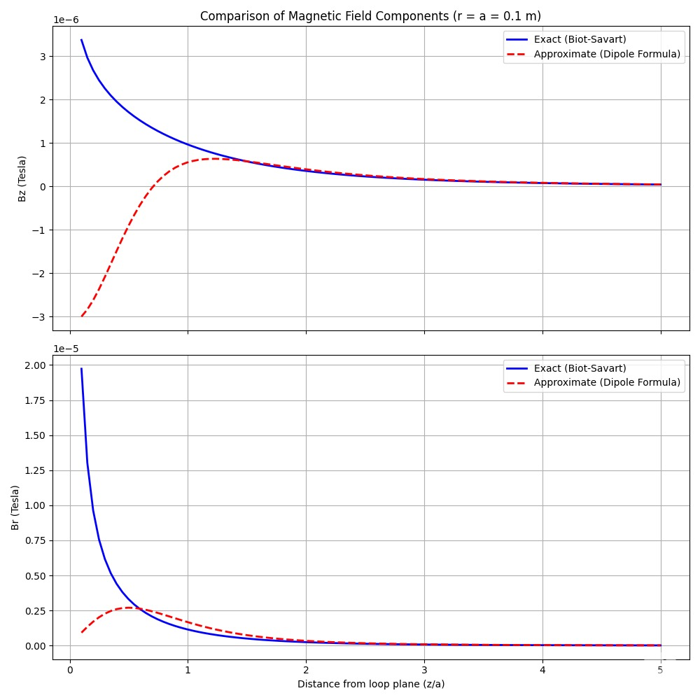
print(Bz_final)Here is the code to compare the result between the far field and the integral result of Biot Savait law.
import numpy as np
import matplotlib.pyplot as plt
from scipy.integrate import quad

# --- 1. Define Constants and Loop Parameters ---
MU_0 = 4 * np.pi * 1e-7  # Permeability of free space (T*m/A)

# Parameters for our physical current loop
a = 0.1  # Radius of the loop (meters)
I = 1.0    # Current in the loop (Amps)
m = I * np.pi * a**2  # Magnetic dipole moment

# --- 2. Dipole Approximation Function ---
def dipole_field(r, z, m):
    """
    Calculates the magnetic field using the point dipole approximation formulas.
    """
    d = np.sqrt(r**2 + z**2)
    # Handle the case where d is very small to avoid division by zero
    if d < 1e-9:
        return 0, 0

    # Br = (mu_0 / 4pi) * (3 * m * r * z) / d**5
    Br_approx = (MU_0 / (4 * np.pi)) * (3 * m * r * z) / d**5

    # Bz = (mu_0 / 4pi) * m * (2*z**2 - r**2) / d**5
    # This is the derived version which has the correct sign on the z-axis.
    Bz_approx = (MU_0 / (4 * np.pi)) * m * (2*z**2 - r**2) / d**5

    return Br_approx, Bz_approx

# --- 3. Exact Biot-Savart Numerical Integration ---
# These are the functions we need to integrate over phi from 0 to 2*pi
def biot_savart_integrands(phi, r, z, a):
    """
    Returns the components of the vector integrand for the Biot-Savart law.
    (dl x R) / |R|^3
    """
    # Denominator |R|^3
    R_mag_cubed = (r**2 + z**2 + a**2 - 2*a*r*np.cos(phi))**(3/2)

    # Numerator (dl x R) components
    # dl = (-a*sin(phi), a*cos(phi), 0)
    # R = (r - a*cos(phi), -a*sin(phi), z)
    # Cross product gives:
    num_x = a * z * np.cos(phi) # This corresponds to the Br component
    num_y = a * z * np.sin(phi) # This should integrate to zero
    num_z = a**2 - a * r * np.cos(phi)

    return num_x / R_mag_cubed, num_y / R_mag_cubed, num_z / R_mag_cubed

def exact_field(r, z, a, I):
    """
    Calculates the exact magnetic field by numerically integrating the Biot-Savart law.
    """
    pre_factor = (MU_0 * I) / (4 * np.pi)

    # Integrate each component of the integrand
    Bx, err_x = quad(lambda phi: biot_savart_integrands(phi, r, z, a)[0], 0, 2*np.pi)
    By, err_y = quad(lambda phi: biot_savart_integrands(phi, r, z, a)[1], 0, 2*np.pi)
    Bz, err_z = quad(lambda phi: biot_savart_integrands(phi, r, z, a)[2], 0, 2*np.pi)

    # Due to symmetry, Bx is our Br, and By should be nearly zero.
    return pre_factor * Bx, pre_factor * Bz

# --- 4. Calculate Fields Along a Line ---
# We will calculate the field at a constant radial distance r, varying z
# A good radial distance to show both components is r = a
r_fixed = a
z_vals = np.linspace(0.01, 5*a, 100) # Calculate from very close to 5x the radius

# Store results
Br_approx_vals, Bz_approx_vals = [], []
Br_exact_vals, Bz_exact_vals = [], []

for z_val in z_vals:
    br_a, bz_a = dipole_field(r_fixed, z_val, m)
    br_e, bz_e = exact_field(r_fixed, z_val, a, I)

    Br_approx_vals.append(br_a)
    Bz_approx_vals.append(bz_a)
    Br_exact_vals.append(br_e)
    Bz_exact_vals.append(bz_e)

# --- 5. Plot the Results ---
fig, (ax1, ax2) = plt.subplots(2, 1, figsize=(10, 10), sharex=True)

# Plot Bz (Vertical Component)
ax1.plot(z_vals/a, Bz_exact_vals, 'b-', label='Exact (Biot-Savart)', linewidth=2)
ax1.plot(z_vals/a, Bz_approx_vals, 'r--', label='Approximate (Dipole Formula)', linewidth=2)
ax1.set_title(f'Comparison of Magnetic Field Components (r = a = {a} m)')
ax1.set_ylabel('Bz (Tesla)')
ax1.legend()
ax1.grid(True)

# Plot Br (Radial Component)
ax2.plot(z_vals/a, Br_exact_vals, 'b-', label='Exact (Biot-Savart)', linewidth=2)
ax2.plot(z_vals/a, Br_approx_vals, 'r--', label='Approximate (Dipole Formula)', linewidth=2)
ax2.set_xlabel('Distance from loop plane (z/a)')
ax2.set_ylabel('Br (Tesla)')
ax2.legend()
ax2.grid(True)

plt.tight_layout()
plt.show()
The Taylor series expansion of 1/|r - r'| is not just a mathematical trick; it is a systematic way of decomposing any arbitrary, complex current distribution into a sum of simpler, idealized sources. Each term in the series represents one of these ideal sources.
For the magnetic vector potential, each term’s field falls off with distance at a different rate.
0th Order: The Magnetic Monopole (Term ~ 1/d)
- Mathematical Origin: This is the
n=0term in the series, where we approximater'as being zero. The integrand for A would be∮ d**l** / d. - Physical Meaning: This term represents the field that would be created by a magnetic monopole—a single, isolated north or south pole.
- Why It’s Zero for a Current Loop: The integral
∮ d**l**around any closed loop is always zero. This is a fundamental geometric fact. Physically, this corresponds to the law that there are no magnetic monopoles (∇ ⋅ B = 0). A current loop has no net “magnetic charge”; for every bit of current moving one way, another bit is moving back elsewhere. Therefore, the monopole term for any real current distribution is always zero.
1st Order: The Magnetic Dipole (Term ~ a/d²)
- Mathematical Origin: This is the
n=1term, the one we carefully isolated in our calculation. It’s the first non-zero term for a current loop. - Physical Meaning: This term represents the source as an idealized magnetic dipole. This is the familiar “tiny current loop” or “infinitesimal bar magnet” model. It captures the primary “lopsidedness” of the magnetic source.
- Dominance at a Distance: Because the monopole term is zero, the dipole term is the most significant part of the magnetic field at large distances. Its field (
B ~ 1/d³) falls off more slowly than any of the higher-order terms, so as you move farther away, the field looks more and more like a pure dipole field. This is why our calculation is so useful.
2nd Order: The Magnetic Quadrupole (Term ~ a²/d³)
- Mathematical Origin: This is the next term in the series, which we truncated with
.removeO(). - Physical Meaning: This term represents the magnetic quadrupole. A quadrupole is a more complex source that can be visualized in a few ways:
- Two identical dipoles placed side-by-side, pointing in opposite directions.
- Two concentric current loops with currents flowing in opposite directions.
- A single current loop that is “squashed” or non-circular (e.g., a square loop).
- When It Matters: The quadrupole moment describes the deviation of the source from a perfect, circular current loop. If a source is constructed with a specific symmetry such that its dipole moment is zero (e.g., two side-by-side coils with opposite currents, used in particle accelerators), then the quadrupole term becomes the dominant far-field behavior.
3rd Order and Higher: Octupoles, etc. (Terms ~ a³/d⁴, …)
- Physical Meaning: These terms represent even more complex source geometries (octupoles, hexadecapoles, etc.). Their fields fall off progressively faster with distance (
B_octupole ~ 1/d⁵, etc.). - When They Matter: These terms are essentially fine-print corrections. They are only important if you are very close to the source, or if you are doing extremely high-precision measurements (like in MRI or particle physics), or if the lower-order moments (dipole, quadrupole) are zero by design.
Summary Table
Taylor Series Order (aⁿ) | Multipole Name | B Field Fall-off | Physical Meaning |
|---|---|---|---|
| n = 0 | Monopole | 1/d² | A single magnetic charge. (Always zero for real sources) |
| n = 1 | Dipole | 1/d³ | A tiny current loop or bar magnet. (The dominant term) |
| n = 2 | Quadrupole | 1/d⁴ | Two opposing dipoles; deviation from a perfect dipole. |
| n = 3 | Octupole | 1/d⁵ | Four opposing dipoles; more complex source geometry. |
The Taylor series is not just a mathematical convenience; it is a physicist’s tool for systematically dissecting a complex reality into a sum of understandable, ideal parts.